This post is also available as an IPython notebook.

I try to be fairly active on the different Stack Exchange sites, and although Stack Overflow is probably undoubtedly the most famous one, I’ve been a big fan and pretty regular contributor over on Code Review. One of the cool things about CR.SE is that they have monthly community challenges where people come up with cool problems, you implement a solution however you want, and you (hopefully) get a useful critique and review of your solution. This month’s problem has to do with rainfall:

A group of farmers has some elevation data, and we’re going to help them understand how rainfall flows over their farmland. We’ll represent the land as a two-dimensional array of altitudes and use the following model, based on the idea that water flows downhill:

• If a cell’s four neighboring cells all have higher altitudes, we call this cell a sink; water collects in sinks.
• Otherwise, water will flow to the neighboring cell with the lowest altitude. If a cell is not a sink, you may assume it has a unique lowest neighbor and that this neighbor will be lower than the cell.
• Cells that drain into the same sink – directly or indirectly – are said to be part of the same basin.

Your challenge is to partition the map into basins. In particular, given a map of elevations, your code should partition the map into basins and output the sizes of the basins, in descending order.

Assume the elevation maps are square. Input will begin with a line with one integer, S, the height (and width) of the map. The next S lines will each contain a row of the map, each with S integers – the elevations of the S cells in the row. Some farmers have small land plots such as the examples below, while some have larger plots. However, in no case will a farmer have a plot of land larger than S = 5000.

Your code should output a space-separated list of the basin sizes, in descending order. (Trailing spaces are ignored.)

This was a really fun problem to solve, and you can find my solution here.

As a whole, this problem really jumps out at me as being a graph problem. We have some plots of land (nodes) and connections between neighboring plots (edges). We want to partition this graph into basins - plots that all drain into the same sink - by removing edges that don’t meet our criteria above.

Let’s make a file to test our implementation against.

In [1]:

with open("simple_rainfall_data.txt", "w") as rainfall_data_file:
    rainfall_data_file.write("""3
1 5 2
2 4 7
3 6 9""")
        
with open("simple_rainfall_data.txt") as rainfall_data_file:
    print(rainfall_data_file.read())

3
1 5 2
2 4 7
3 6 9

Once we’ve partitioned that data into our basins, we’d have something like this:

A* A B*
A  A B
A  A A

Where $A$ and $B$ are basins, and $A$ and $B$ are the sinks.

Lets get started with some code!

After we’ve imported the tools we need, we first need to load in our data and build our initial graph. This has no removed edges; we assume that all plots with a neighbor on the cardinal axes have an edge between them.

I’m using a super cool library NetworkX to make my graphs. I’m using a relatively outdated version, but the general concept should be doable with pretty much any version.

One of the nicest features about NetworkX is that it doesn’t require you to use its own node or edge data structures - any valid Python object works. Internally it uses lots of dictionaries so you can add arbitrary attributes to nodes and edges as well, which is helpful for us. For now we’ll consider a node the $(x, y)$ coordinates of the plot, and we’ll keep track of a few attributes of our plot as well: the plot’s elevation and the basin it falls in. To start, the basin will just be the current plot - we don’t know anything more at this point.

We can also add the edges at the same time, but we need to be a little careful because adding an edge in NetworkX will create any missing nodes. To avoid that problem we make each node responsible for creating the edge to its neighbors at $(x - 1, y)$ and $(x, y - 1)$ as long as the neighbor is already part of the graph.

I also skip the header line - thanks to the glory of Python I don’t need to worry about manual allocation or anything like that, and it also makes the code more flexible. Whatever size input we get, we can handle. I also intentonally didn’t put in any validation of the input file; I didn’t think that it would be worthwhile for this example.

Note: These functions are going to change a bit over the course of this post as I realize some things I’m missing.

In [2]:

import networkx as nx

def build_topography(filename):
    with open(filename) as elevation_data:
        lines = iter(elevation_data)
        next(lines)

        topography = nx.Graph()

        for row_index, row in enumerate(lines):
            for plot_index, elevation in enumerate(map(int, row.split())):
                plot = (row_index, plot_index)
                topography.add_node(
                    plot,
                    elevation=elevation,
                    basin=plot
                )
                add_edges(topography, plot)

    return topography

def add_edges(topography, plot):
    above_node = (plot[0] - 1, plot[1])
    left_node = (plot[0], plot[1] - 1)
    if above_node in topography:
        topography.add_edge(plot, above_node)
    if left_node in topography:
        topography.add_edge(plot, left_node)

I want a convenient way to be able to visualize my graphs as they are made, so I wrote a little utility function. As it turns out drawing a graph is pretty hard, so the output might not always be quite as pretty as I’d like. Usually running it a few times will give you something mostly pretty. This may not be ultra-friendly to any color-blind folks reading this; I apologize in advance.

In [3]:

import matplotlib.pyplot as plt
%matplotlib inline

def get_label(topography, node):
    n_dict = topography.node[node]
    return "{} - {}".format(n_dict['basin'], n_dict['elevation'])

def display_graph(topography):
    # Todo: Work out colors for color-blindedness
    labels = {node : get_label(topography, node) for node in topography.nodes()}
    kwargs = {
        'with_labels': True,
        'layout': nx.shell_layout(topography),
        'labels': labels
    }

    nx.draw(topography, **kwargs)
    plt.draw()
    plt.show()
    
topography = build_topography("simple_rainfall_data.txt")
display_graph(topography)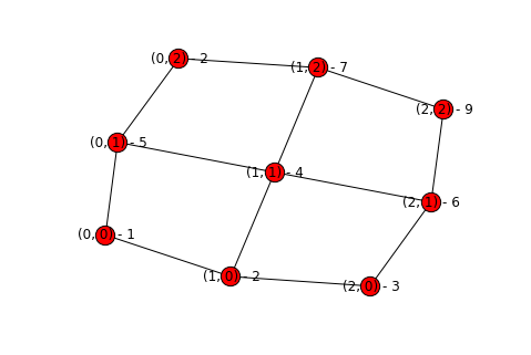

At this point we have a workable graph with all of the pertinent information - the elevations and the potential connections. Now we need to remove edges to get to the final graph.

There are a few ways we could try to approach this problem:

1. Iterate over every node in whatever order they happen to be in and remove certain edges.
2. Find the sinks, then work our way up
3. Find the highest points, then work our way down.

I ended up choosing option 3 - here’s why.

The first option would be a little tricky; for some arbitrary node we want to remove irrelevant edges. Irrelevant edges are ones where water doesn’t pass, so any neighbor with a higher elevation that itself that has another neighbor with a lower elevation (than the current node), and any neighbor with a lower elevation that is still higher than another one of the neighbor’s elevations. Pseudocoded out, that would look something like this

for each node in topography
    for each neighbor of the node
        if neighbor's elevation is greater than node's, and neighbor's lowest
neighbor is not node
            remove edge between neighbor and node
        else if neighbor's elevation is lower than node's, but node has another
neighbor with an even lower elevation
            remove edge between neighbor and node

That wouldn’t necessarily be awful to do, but it is a little tricky to conceptualize and there are a few gotchas as well.

The second option is also tricky - we end up having basically the same problems as with option one, except it isn’t an arbitrary node. One extra wrinkle is that we can have multiple “parent” nodes for any given node, while we have at most one “child” node. This ends up lending itself to the third option quite nicely.

If we have a list of the plots, sorted from highest to lowest elevation, then we have a very simple algorithm to implement

for each node in sorted_nodes
    let edges be the neighbors of node
    if there are any edges
        find the edge to the neighbor with the lowest implementation below
node's
        if there is such an edge
            mark this node as the other node's parent
            mark the other node as this node's child
        remove all edges from this node that are neither a parent nor a child
edge

Because we start at the very top, we will know all of the parents for a given node from the beginning. Then it is a simple task to figure out the least neighbor, and then remove all of the extra nodes.

In order to do this, we need to build up a sorted list of the nodes in the graph. This is easy to do while we’re building the graph, especially if we use the bisect stdlib module. It is especially nice because it performs a binary search to find the insertion point of a given node, which means our sorting ends up happening in O(log(n)) time (ignoring the cost of inserting items, which is probably around O(n)).

We also want to keep track of a node’s parents from when we start, so we’ll add that attribute to our graph as well.

We also use namedtuple and total_ordering to remove more cruft - Python really made this easy by including all of the batteries we need.

In [4]:

from collections import namedtuple
from functools import total_ordering
import bisect


@total_ordering
class PlotData(namedtuple('PlotData', 'plot elevation')):

    def __lt__(self, other):
        return self.elevation < other.elevation

    def __eq__(self, other):
        return self.elevation == other.elevation

def build_topography(filename):
    with open(filename) as elevation_data:
        lines = iter(elevation_data)
        next(lines)

        topography = nx.Graph()
        sorted_plots = []

        for row_index, row in enumerate(lines):
            for plot_index, elevation in enumerate(map(int, row.split())):
                plot = (row_index, plot_index)
                add_node(topography, sorted_plots, plot, elevation)
                add_edges(topography, plot)

    return topography, reversed(sorted_plots)

def add_node(topography, sorted_plots, plot, elevation):
    data = PlotData(plot, elevation)
    bisect.insort(sorted_plots, data)
    topography.add_node(
        plot,
        elevation=elevation,
        basin=plot,
        parents=[]
    )

Now that we have fixed how we build up our graph, we can actually process it.

In [5]:

def process_topography(topography, sorted_nodes):
    for node in sorted_nodes:
        node = node.plot
        edges = topography[node]
        if edges:
            min_elevation = topography.node[node]['elevation']
            basin = node
            parents = topography.node[node]['parents']
            for connected_node in edges:
                elevation = topography.node[connected_node]['elevation']
                if elevation < min_elevation:
                    min_elevation = elevation
                    basin = connected_node
            topography.node[node]['basin'] = basin
            topography.node[basin]['parents'].append(node)
            topography.node[basin]['parents'].extend(parents)
            edges_to_remove = [connected_node
                               for connected_node in edges
                               if connected_node != basin and
                                  connected_node not in parents]
            for edge_to_remove in edges_to_remove:
                topography.remove_edge(node, edge_to_remove)
                
topography, sorted_plots = build_topography("simple_rainfall_data.txt")
process_topography(topography, sorted_plots)
display_graph(topography)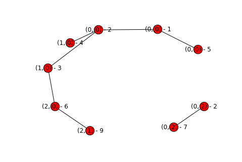

Hooray! We’ve successfully partitioned our graph and remove all of the extraneous edges. A few things to note about our graph:

1. It’s acyclic - if we had a cycle that would mean we haven’t correctly removed all of our edges, as there should only be one path from a given point to it’s associated sink.
2. Each basin is disconnected from the others - if you don’t remember your graph theory then you can read up on connectivity, but basically each connected sub-component of the graph is a basin.

There are still some weird aspects about this solution that I’ll touch on in a bit, but first we need to actually meet the criteria of the problem - output a space-separated list of the size of each basin in descending order. This ends up being really easy - NetworkX has some nice methods to get the connected sub- components of a graph.

In [6]:

def get_basin_sizes(connected_components):
    return (
        len(component)
        for component in sorted(connected_components, key=len, reverse=True)
    )

for basin in get_basin_sizes(nx.connected_components(topography)):
    print basin,

7 2

And voila!

Now let’s talk about some of the weird things. If we look at our last graph again, you’ll notice that the basins they’re labelled with aren’t quite right. This isn’t necessarily a problem - no requirement exists that each node knows its own basin - but it would be a nice thing to fix. This ends up being pretty easy:

for each node in the graph
    if node is a sink
        update all of node's parents' basins to be node

In [7]:

def fix_basins(topography):
    for node in topography.nodes():
        if is_sink(topography, node):
            for parent in topography.node[node]['parents']:
                topography.node[parent]['basin'] = node

def is_sink(topography, node):
    connected_nodes = topography[node]
    parents = topography.node[node]['parents']
    return all(connected in parents for connected in connected_nodes)

fix_basins(topography)
display_graph(topography)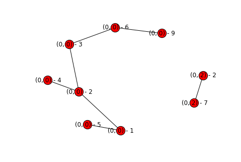

We can now see that each node has its own basin appropriately labeled. This then makes it even easier for us to add colors for each component! We can just get the connected components again, and look at the basin of the first one. Then just map from basin to color, and update how we draw our graphs.

In [8]:

import numpy as np

def get_basin_colors(topography):
    connected_components = list(nx.connected_components(topography))
    colors = np.linspace(0, 1, len(connected_components))
    return {
        topography.node[component[0]]['basin'] : color
        for component, color in zip(connected_components, colors)
    }


def display_graph(topography):
    labels = {node : get_label(topography, node) for node in topography.nodes()}
    color_dict = get_basin_colors(topography)
    colors = [color_dict[topography.node[node]['basin']] for node in topography.nodes()]
    
    kwargs = {
        'with_labels': True,
        'layout': nx.shell_layout(topography),
        'labels': labels,
        'node_color': colors
    }
    
    nx.draw(topography, **kwargs)
    plt.draw()
    plt.show()
    
display_graph(topography)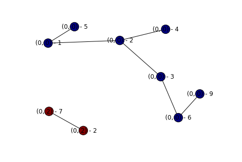

We now have a nice and pretty solution to our graph problem! I’ll update this post later once I get feedback on my solution (either in the comments below, or over on CR.SE) to discuss things that work well, and things that don’t.

My biggest concern about my solution is scalability - lots of graph algorithms aren’t cheap, and if we end up with large tracts of land, i.e. $5000 x 5000$ (the largest size possible according to the problem) then I don’t know how well my solution scales. I haven’t gotten around to writing a function to generate new arbitrary-sized plots of land, but once I do I’ll be sure to test how my solution scales.